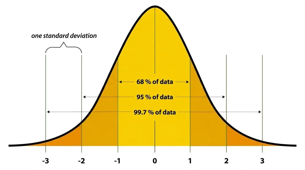

TL;DR: Standard deviation (SD) is a single number that tells you how spread out your data is. A small SD means values cluster tightly around the average; a large SD means they scatter far and wide. You calculate it in five steps: find the mean, subtract the mean from each data point, square those differences, average them (divide by N for a population, or n−1 for a sample), then take the square root. The sample formula uses n−1 (called Bessel’s correction) because the sample mean slightly underestimates the true spread. For normally distributed data, the empirical rule says ~68% of values fall within 1 SD, ~95% within 2 SD, and ~99.7% within 3 SD of the mean.
What is standard deviation, in plain English?
Imagine two basketball players. Player A scores 18, 19, 20, 21, and 22 points across five games. Player B scores 5, 12, 20, 28, and 35. Both average exactly 20 points per game — but they’re nothing alike. Player A is reliable and consistent. Player B is thrilling but wildly unpredictable. The mean (average) hides that difference completely. Standard deviation exposes it.
In statistics, standard deviation meaning boils down to this: it measures the average distance of your data points from their mean. It’s the most common way to describe variability or dispersion in a set of numbers. The U.S. National Library of Medicine defines it as a measure of “how dispersed the data is in relation to the mean” — low SD means data clusters tightly, high SD means it spreads out.
Here’s the intuition in two sentences:
- Low SD: Most values sit close to the average. Think of heights in a third-grade classroom — everyone’s roughly the same size.
- High SD: Values scatter widely. Think of annual incomes in a big city — a few billionaires pull the spread way up.
Standard deviation is never negative. If every number in your dataset is identical, SD equals zero. As your data gets more spread out, SD grows. And crucially, SD shares the same units as your original data — if you measure heights in inches, SD is also in inches. That’s the main reason people prefer it over variance (which lives in squared units).
The standard deviation formula (and why there are two of them)
The standard deviation formula looks scarier than it is. Once you break it into pieces, it’s just five arithmetic steps. But you need to pick the right version first — and this is where almost everyone gets tripped up.
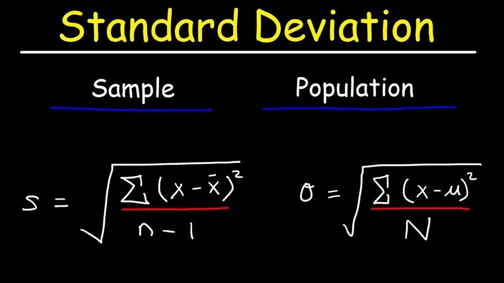
Population standard deviation (σ, “sigma”): Use this when your data includes every single member of the group you care about (a census). Divide by N.
$$\sigma = \sqrt{\frac{\sum(x_i – \mu)^2}{N}}$$
Sample standard deviation (s): Use this when your data is a sample drawn from a larger population, and you want to estimate that population’s true spread. Divide by n−1.
$$s = \sqrt{\frac{\sum(x_i – \bar{x})^2}{n – 1}}$$
Here’s what every symbol means:
| Symbol | What it stands for |
|---|---|
| σ or s | Population SD (Greek sigma) or sample SD (italic s) |
| xᵢ | Each individual data point |
| μ or x̄ | Population mean (mu) or sample mean (“x-bar”) |
| Σ | Uppercase sigma — “sum up everything that follows” |
| N or n | Total number of data points (capital N = population, lowercase n = sample) |
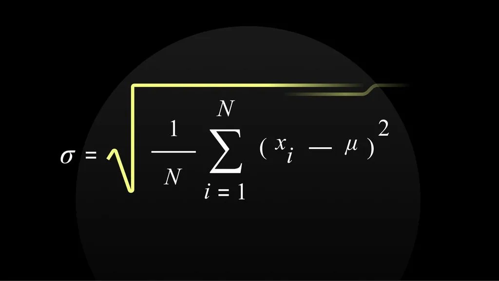
The only real difference between the two formulas is the denominator: N vs. n−1. Everything else is identical. The Math Doctors walk through the full derivation of both formulas (plus a shortcut “computational formula” that avoids calculating the mean first) in their deep-dive on standard deviation formulas.
How to find standard deviation in 5 steps
Let’s do this by hand with a tiny dataset so you see exactly where the number comes from. Real statisticians never calculate this by hand — they use software — but working through it once is how the concept clicks. Khan Academy’s step-by-step guide uses the same five-step approach, and it’s the fastest way to build intuition.
Our dataset: Five test scores — 72, 85, 79, 91, 68.
Step 1: Find the mean (average)
Add them up and divide by how many there are.
Mean = (72 + 85 + 79 + 91 + 68) ÷ 5 = 395 ÷ 5 = 79
If you need to double-check the mean, a quick mean median mode calculator does it in a second.
Step 2: Subtract the mean from each data point (the “deviations”)
This tells you how far each score sits from the average.
| Score (xᵢ) | Deviation (xᵢ − mean) |
|---|---|
| 72 | 72 − 79 = −7 |
| 85 | 85 − 79 = +6 |
| 79 | 79 − 79 = 0 |
| 91 | 91 − 79 = +12 |
| 68 | 68 − 79 = −11 |
Notice something: the deviations add up to zero (−7 + 6 + 0 + 12 − 11 = 0). That always happens — it’s how the mean is defined. So we can’t just average the deviations; they’d cancel out to zero and pretend there’s no spread at all. We need the next step.
Step 3: Square each deviation
Squaring does two clever things at once: it turns every negative number positive (so points above and below the mean both count), and it punishes large deviations more than small ones (a deviation of 12 contributes 144, while a deviation of 6 contributes only 36).
| Deviation | Squared deviation |
|---|---|
| −7 | 49 |
| +6 | 36 |
| 0 | 0 |
| +12 | 144 |
| −11 | 121 |
Step 4: Average the squared deviations — this is the variance
Sum of squared deviations = 49 + 36 + 0 + 144 + 121 = 350.
- Population variance (divide by N = 5): 350 ÷ 5 = 70
- Sample variance (divide by n−1 = 4): 350 ÷ 4 = 87.5
Step 5: Take the square root — this is the standard deviation
- Population SD: √70 ≈ 8.37 points
- Sample SD: √87.5 ≈ 9.35 points
So for these five test scores, the standard deviation is roughly 8.4 (if these five students are the whole group) or 9.4 (if they’re a sample standing in for a larger class). Either way, scores typically land about 8–9 points away from the 79 average.
Why divide by n−1? Bessel’s correction, explained without the math
This is the single most common “why?” question in introductory stats. If you have n data points, why not just divide by n?
Here’s the plain-English version. When you work with a sample, you don’t know the true population mean μ — you only know the sample mean x̄. And here’s the catch: the sample mean is, by definition, the point that minimizes the sum of squared deviations. No other number produces a smaller sum. So when you measure deviations from x̄ instead of the true μ, you systematically underestimate the true spread. Dividing by n−1 instead of n inflates the result just enough to correct that bias.
This correction is named Bessel’s correction, after Friedrich Bessel, the German astronomer who spotted it in 1815 while analyzing errors in astronomical observations. A Stanford derivation puts it precisely: using the sample mean rather than the true population mean causes a systematic underestimation, and dividing by n−1 yields an unbiased estimator of the variance.
A quick rule of thumb:
- Divide by N when your data IS the whole population (e.g., the heights of all 9 students in a class).
- Divide by n−1 when your data is a sample and you’re estimating a larger population (the vast majority of real-world cases).
- The difference shrinks as n grows — with 1,000 data points, dividing by 1000 vs 999 barely changes the result. With 5 data points, it matters a lot.
Standard deviation vs. variance: what’s the difference?
These two are close cousins, and people mix them up constantly. The relationship is dead simple:
Standard deviation = √variance
Variance = (standard deviation)²
Variance is the number you get at Step 4 — the average of the squared deviations. Standard deviation is the square root of that number (Step 5). So why bother taking the square root at all? Because variance lives in squared units, which are meaningless to humans. If your data is test scores, variance is in “points squared” — a unit nobody can visualize. Square-root it and you’re back in plain old points, which you can immediately compare to the mean.
JMP’s statistics knowledge portal sums it up cleanly: “Age in years is simpler to think about than squared age in years.” That’s why every research paper reports mean ± SD, not mean ± variance.
Interpreting standard deviation: the empirical rule (68–95–99.7)
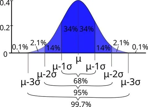
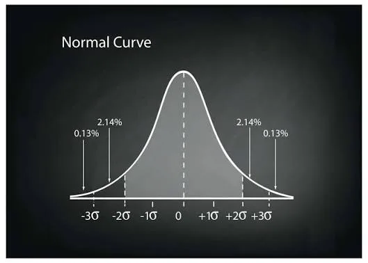
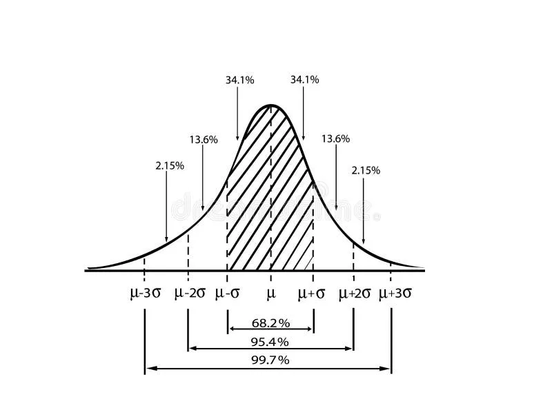
A raw SD number doesn’t mean much until you put it in context. For data that follows a normal distribution (the classic bell curve — heights, test scores, measurement errors, many biological traits), the empirical rule turns SD into a precise probability cheat sheet:
| Range | % of data you’d expect there |
|---|---|
| Mean ± 1 SD | ~68% of values |
| Mean ± 2 SD | ~95% of values |
| Mean ± 3 SD | ~99.7% of values |
OpenStax’s Introductory Statistics confirms the rule: for a normally distributed variable with mean μ and standard deviation σ, roughly 68% of values fall within ±1σ, 95% within ±2σ, and 99.7% within ±3σ.
Let’s make it real. Adult women in the U.S. have a mean height of about 64.5 inches with an SD of about 2.5 inches. Applying the rule:
- ~68% of women are between 62″ and 67″ (5′2″ to 5′7″)
- ~95% are between 59.5″ and 69.5″ (4′11.5″ to 5′9.5″)
- ~99.7% are between 57″ and 72″ (4′9″ to 6′0″)
That’s the power of one small number: mean + SD lets you reconstruct almost the entire distribution. If a value sits more than 2 SD from the mean, it’s in the rarest 5% — a genuine outlier. More than 3 SD? You’re in the 0.3% tail, which is almost unheard of. Particle physicists use a 5-sigma threshold (5 SD from the mean) to claim a discovery — that’s a one-in-3.5-million fluke.
Where standard deviation actually gets used (it’s everywhere)
You encounter standard deviation constantly, even when you don’t see the symbol.
- Finance: Investors call standard deviation of returns “volatility.” A stock with high SD swings wildly — high risk, high potential reward. A bond fund with low SD is boring but stable. Sharpe ratios and modern portfolio theory are built on it.
- Health & medicine: Clinical trials report “mean ± SD” for blood pressure, cholesterol, drug response. The NLM’s health statistics guide uses SD to describe how patient heights and lab values distribute.
- Quality control (Six Sigma): Manufacturers measure SD of part dimensions. “Six Sigma” quality means defects sit beyond 6 SD from the mean — 3.4 defects per million opportunities.
- Sports analytics: A quarterback with a low SD in passer rating is consistent; a high-SD one is boom-or-bust. Same for batting averages, golf scores, and marathon times.
- Weather & climate: SD of daily temperatures tells you how much a location’s weather swings. Coastal cities have low SD; continental interiors have high SD.
- Education: Standardized tests (SAT, GRE, IQ) are deliberately scaled so scores have a fixed mean and SD (e.g., IQ: mean 100, SD 15). A score of 130 is exactly 2 SD above average — top ~2.5%.
Common mistakes (and when NOT to use standard deviation)
Standard deviation is powerful, but it’s not a universal tool. Watch for these traps:
- Outliers distort it heavily. Because you square deviations, one extreme value can dominate the sum. In JMP’s heart-rate example, adding a single outlier (140 bpm) jumped the SD from 11.8 to 28.6. If you have outliers, report the median and interquartile range (IQR) instead — they’re robust.
- Don’t use it on ordinal or nominal data. SD only makes sense for continuous numerical data (height, weight, time, money). Calculating SD of “Strongly Disagree = 1, Strongly Agree = 5” survey responses gives you a number, but it’s mathematically meaningless. Use a frequency table instead.
- Skewed data breaks the empirical rule. The 68–95–99.7 rule assumes a normal (symmetric) bell curve. For skewed data (incomes, house prices, hospital wait times), mean ± SD misleads. Use median and percentiles.
- Don’t delete outliers just because they’re extreme. Investigate first. If an outlier is a data-entry error, fix it. If it’s real, keep it — or report results both with and without it. Never silently drop values.
- Don’t confuse SD with standard error. Standard deviation describes spread within a sample. Standard error (SD ÷ √n) describes how precisely you’ve estimated the mean. They answer different questions.
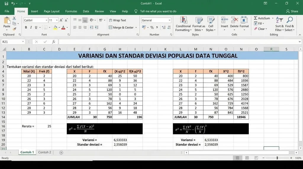
How to calculate standard deviation in Excel, Google Sheets, and online
Nobody does this by hand anymore. Here are the functions you actually need:
| Tool | Sample SD (n−1) | Population SD (N) |
|---|---|---|
| Excel / Google Sheets | =STDEV.S(range) | =STDEV.P(range) |
| Old Excel (pre-2010) | =STDEV(range) | =STDEVP(range) |
| Python (pandas) | df['col'].std() (default ddof=1) | df['col'].std(ddof=0) |
| R | sd(x) (sample by default) | sqrt(mean((x-mean(x))^2)) |
| TI-84 calculator | 1-Var Stats → Sx (sample) / σx (population) | same menu |
The most common Excel mistake is using STDEV.P when you meant STDEV.S — or vice versa. Double-check the denominator. If you just want a fast answer without opening a spreadsheet, our standard deviation calculator handles both population and sample formulas, and it returns variance, mean, and sum of squares alongside SD.
A quick comparison: SD vs. range vs. IQR
Standard deviation isn’t the only way to measure spread. Here’s when to reach for which:
| Measure | How it’s calculated | Best for | Robust to outliers? |
|---|---|---|---|
| Range | Max − min | Quick, rough idea | No |
| Interquartile range (IQR) | 75th percentile − 25th percentile | Skewed data, outliers | Yes |
| Standard deviation | √(average squared deviation from mean) | Symmetric, continuous data; further stats work | No |
| Variance | SD² | Mathematical derivations | No |
If your data is clean and roughly bell-shaped, mean ± SD is the gold standard report. If it’s skewed or full of outliers, median (IQR) is more honest.
Frequently Asked Questions
What is standard deviation in statistics?
Standard deviation is a measure of spread — it quantifies how far data points typically lie from their mean. A low SD means values cluster tightly; a high SD means they scatter widely. It’s the square root of the variance and shares the same units as the original data.
What is the standard deviation formula?
For a population: σ = √(Σ(xᵢ − μ)² / N). For a sample: s = √(Σ(xᵢ − x̄)² / (n − 1)). The only difference is dividing by N (population) vs. n−1 (sample, Bessel’s correction).
How do I find standard deviation step by step?
Five steps: (1) calculate the mean, (2) subtract the mean from each data point, (3) square each difference, (4) average the squared differences (divide by N or n−1) to get variance, (5) take the square root. That’s your standard deviation.
Why do we use n−1 instead of n?
Because the sample mean (x̄) minimizes the sum of squared deviations, which systematically underestimates the true population spread. Dividing by n−1 (Bessel’s correction) corrects that bias and gives an unbiased estimate of the variance. Use N only when you have data for the entire population.
What’s a “good” standard deviation?
There’s no universal threshold — it depends on context. A 2-inch SD for human heights is large; a 2-inch SD for bridge spans is tiny. To judge it, compare SD to the mean (that ratio is the coefficient of variation, CV) or use the empirical rule if your data is normal.
What does 1 standard deviation from the mean mean?
For normally distributed data, about 68% of values fall within ±1 SD of the mean. ±2 SD covers ~95%, and ±3 SD covers ~99.7%. A value beyond 2 SD is unusual; beyond 3 SD is rare.
Can standard deviation be zero?
Yes — if every value in your dataset is identical, there’s no spread, and SD equals zero. Standard deviation can never be negative.
Should I use sample or population standard deviation?
Use population (N) only when your data includes every member of the group you’re studying. In almost every real-world case — surveys, experiments, A/B tests — you’re working with a sample, so use n−1.
Final thought
Standard deviation looks like a scary formula, but it’s really just one idea: how far, on average, does my data wander from the middle? Master the five steps, remember the n−1 rule for samples, and apply the 68–95–99.7 rule when your data is normal, and you’ll have 90% of what you need to read any research paper, any sports stat line, or any financial report. The other 10% is knowing when not to use it — outliers, skewed data, and non-numeric scales.