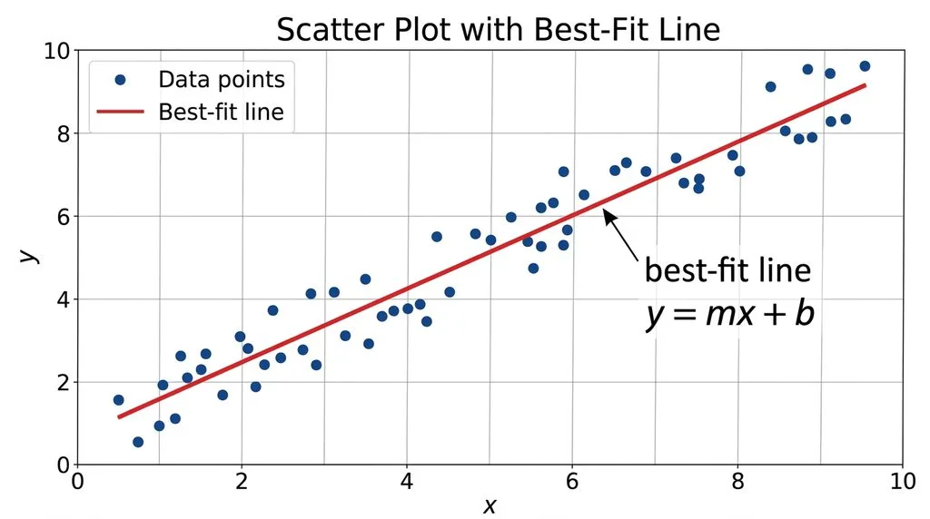

TL;DR: A linear regression equation — also called a regression line or line of best fit — is the straight line ŷ = b₀ + b₁x (or y = mx + b) that sits closest to all your data points at once. You find it with the least squares method, which minimizes the sum of the squared vertical distances (residuals) from each point to the line. The slope formula is m = (nΣxy − ΣxΣy) / (nΣx² − (Σx)²) and the intercept is b = ȳ − mx̄. The line always passes through the point (x̄, ȳ). Use it to predict y from x, but only when the relationship is roughly linear, errors are independent with constant variance, and outliers aren’t driving the result.
What is a linear regression equation, anyway?
Picture this: you track how many hours five students studied for a test and the scores they got. You plot the five dots on a graph. Some dots sit high, some low, but you can see a trend — more hours tends to mean a better score. Now ask: what single straight line summarizes that trend best? That line is your regression line, and its equation is your linear regression equation.
In plain English, linear regression answers two questions at once:
- Is there a straight-line relationship between X and Y?
- If yes, what’s the equation of that line, and how well does it fit?
Once you have the equation, you can plug in any X and get a predicted Y. That’s why every field from finance to medicine to machine learning uses it — it’s the simplest predictive model in statistics, and it’s been the workhorse of data analysis for over 200 years.
The word “regression” has a charming origin. In 1886, Sir Francis Galton studied parents’ heights and their children’s heights and noticed that very tall parents tended to have children who were shorter than them — closer to the average. He called this “regression toward the mean,” and the name stuck to the whole method. Legendre and Gauss had already developed the least squares math around 1805 to predict planetary orbits, and Adolphe Quetelet later brought it into the social sciences. Wikipedia’s linear regression article covers that full history if you want the deep dive.
There are two flavors worth knowing up front:
- Simple linear regression: One X predicts one Y. Equation: ŷ = b₀ + b₁x. This is what 90% of people mean when they say “linear regression,” and it’s what this guide covers.
- Multiple linear regression: Several X’s predict one Y. Equation: ŷ = b₀ + b₁x₁ + b₂x₂ + … + bₖxₖ. Same idea, more variables.
The linear regression formula: every symbol, explained
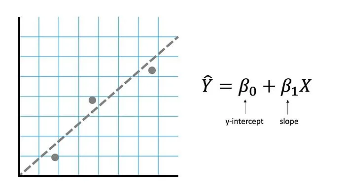
The standard deviation of a single variable tells you spread; the regression line tells you direction. Here’s the equation you’ll see in every textbook, written two equivalent ways:
Algebra class version: y = mx + b
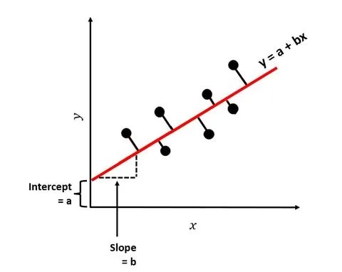
Statistics version: ŷ = b₀ + b₁x (or ŷ = a + bx)
| Symbol | What it means |
|---|---|
| ŷ (“y-hat”) | The predicted value of Y for a given X |
| x | The independent variable (the one you control or observe) — always on the horizontal axis |
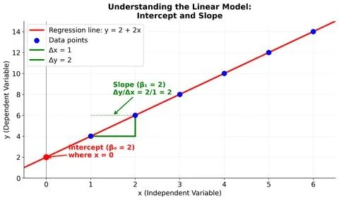
| b₁ or m | Slope — how much Y changes, on average, for every one-unit increase in X |
| b₀ or b or a | Y-intercept — the predicted value of Y when X = 0; where the line crosses the vertical axis |
| n | Number of data points |
| Σ | Uppercase sigma — “add up everything that follows” |
And here are the two formulas that actually produce m and b — the ones you’ll use by hand:
Slope:
$$m = \frac{n\sum xy – (\sum x)(\sum y)}{n\sum x^2 – (\sum x)^2}$$
Intercept:
$$b = \bar{y} – m\bar{x}$$
…where x̄ is the mean of the X values and ȳ is the mean of the Y values. Notice what the intercept formula tells you: the regression line always passes through the point (x̄, ȳ) — the center of your data. OpenStax’s Statistics textbook confirms this property in its chapter on the regression equation, and it’s the fastest sanity check on any line you calculate.
There’s an equivalent “deviation form” of the slope formula you’ll see in more advanced stats: m = Σ(x − x̄)(y − ȳ) / Σ(x − x̄)². It gives exactly the same answer — it’s just written in terms of distances from the means instead of raw sums. Both are correct. Use whichever you find easier.
How to calculate the line of best fit by hand in 5 steps
Nobody does this by hand for real data — you’ll use Excel, a calculator, or Python. But working through one tiny example by hand is how the formula stops looking like hieroglyphics and starts making sense. The Carleton College math guide uses the same five-step method with volcano data, and a Reddit thread on r/learnmath confirmed exactly what students keep asking: the “eyeball a line through two points” trick you may have learned is not the real method — the real method is least squares, and it’s meticulous but mechanical.
Our dataset: Hours studied (X) vs. test score (Y) for 5 students.
| Student | Hours (x) | Score (y) |
|---|---|---|
| A | 1 | 55 |
| B | 2 | 62 |
| C | 3 | 70 |
| D | 4 | 78 |
| E | 5 | 85 |
Step 1: Find the means and build your three helper columns
For every (x, y) pair, compute x² and xy. Add columns to your table — this keeps you organized. A quick mean median mode calculator can double-check your averages.
| x | y | x² | xy |
|---|---|---|---|
| 1 | 55 | 1 | 55 |
| 2 | 62 | 4 | 124 |
| 3 | 70 | 9 | 210 |
| 4 | 78 | 16 | 312 |
| 5 | 85 | 25 | 425 |
| Σx = 15 | Σy = 350 | Σx² = 55 | Σxy = 1126 |
n = 5. x̄ = 15/5 = 3. ȳ = 350/5 = 70.
Step 2: Calculate the slope (m)
Plug into the slope formula:
Numerator = nΣxy − (Σx)(Σy) = 5(1126) − (15)(350) = 5630 − 5250 = 380
Denominator = nΣx² − (Σx)² = 5(55) − (15)² = 275 − 225 = 50
m = 380 / 50 = 7.6
So every extra hour of study predicts, on average, a 7.6-point increase in test score.
Step 3: Calculate the intercept (b)
b = ȳ − mx̄ = 70 − (7.6)(3) = 70 − 22.8 = 47.2
Step 4: Write the regression equation
ŷ = 47.2 + 7.6x
That’s your line of best fit.
Step 5: Use it to predict, and check it passes through (x̄, ȳ)
Predict the score for someone who studied 3.5 hours: ŷ = 47.2 + 7.6(3.5) = 47.2 + 26.6 = 73.8.
Sanity check: plug in x̄ = 3 → ŷ = 47.2 + 22.8 = 70 = ȳ. ✓ The line passes through the center of the data, as it must.
Why “least squares”? The genius of squaring the residuals
Why do we square things? Why not just find the line that minimizes the average distance from the points? Here’s the problem: distances above the line are positive, distances below are negative, and if you just add them up, they cancel to zero — every line would look equally good. Squaring does two clever things:
- It makes every residual positive, so points above and below the line both count.
- It punishes big misses harder than small ones — a point 10 units off contributes 100, while a point 2 units off contributes only 4.
A residual is the vertical gap between an actual data point and the line: residual = y − ŷ. The least squares method finds the unique line that makes the sum of all squared residuals as small as mathematically possible. There’s a closed-form solution (the formulas above), so no guessing, no iteration — you get the exact best line in one calculation.
One consequence of squaring: outliers have outsized power. A single wild point can yank the whole line toward it. That’s why you always plot your data first — a scatter plot takes 30 seconds and saves you from a wildly wrong conclusion.
Interpreting your line: slope, intercept, r, and R²
The numbers alone don’t mean much until you interpret them. Here’s the full toolkit:
- Slope (b₁): The direction and size of the relationship. Positive slope → Y rises with X. Negative slope → Y falls as X rises. Slope = 7.6 in our example means “each additional hour associates with +7.6 points, on average.” Important: this is association, not proof of causation.
- Intercept (b₀): Predicted Y when X = 0. Sometimes meaningful (a student who studied 0 hours scores ~47), sometimes mathematically real but practically meaningless (a house with 0 square feet costs negative dollars — extrapolation beyond your data range is dangerous).
- Correlation coefficient (r): From −1 to +1. Tells you strength and direction of the linear relationship. r = +1 is a perfect upward line, r = 0 is no linear relationship, r = −1 is a perfect downward line. Slope and r always share the same sign. You can compute it instantly with a correlation calculator.
- R-squared (R²): From 0 to 1. The percentage of variation in Y that the line explains. R² = 0.81 means 81% of the variation in test scores is explained by study hours. For simple linear regression, R² = r². Khan Academy’s regression lessons walk through how to interpret R² in context.
Quick rule of thumb for r (it varies by field):
| |r| | Strength of linear relationship |
|---|---|
| 0.0–0.3 | Weak or none |
| 0.3–0.7 | Moderate |
| 0.7–1.0 | Strong |
In our study-hours example, r ≈ 0.995 and R² ≈ 0.99 — an almost perfect fit, because I built the data that way. Real-world data is messier.
The assumptions behind linear regression (and Anscombe’s warning)
Ordinary least squares regression gives you a line every single time, even when a line is the wrong model. For the results to be trustworthy — especially for p-values, confidence intervals, and predictions — four assumptions should roughly hold. People remember them with the mnemonic LINE:
- L — Linearity: The true relationship between X and Y is roughly a straight line. Plot your data. If you see a curve, linear regression will mislead you.
- I — Independence: Each residual doesn’t predict the next. This fails most often in time-series data (today’s error correlates with yesterday’s).
- N — Normality: Residuals are approximately normally distributed around zero. Matters mostly for small samples and for p-values.
- E — Equal variance (homoscedasticity): The spread of residuals stays constant across all X values. If the scatter “fans out” as X grows (heteroscedasticity), your prediction intervals are wrong.
These four conditions are standard across regression texts and LibreTexts’ diagnostics chapter lays them out cleanly alongside residual-plot guidance.
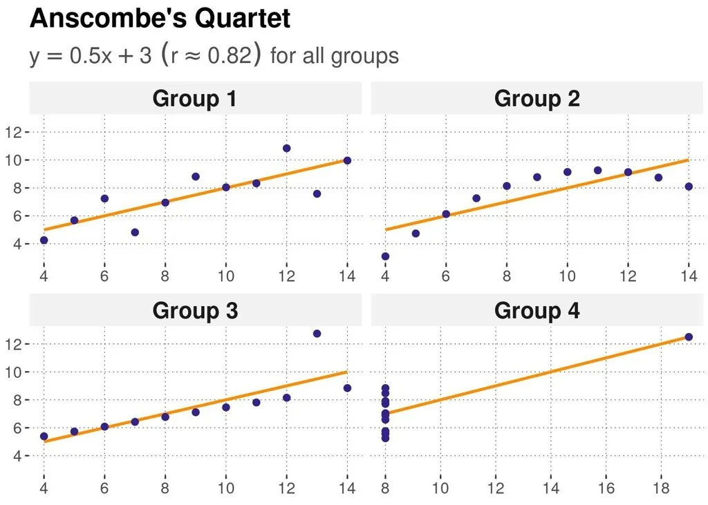
And here’s the single most important picture in all of statistics: Anscombe’s Quartet. In 1973, statistician Francis Anscombe published four datasets that have identical means, variances, correlation coefficients (r ≈ 0.82), and regression lines (y = 3 + 0.5x). But when you plot them, they’re completely different — one is a clean linear cloud, one is a curve, one has a single outlier tilting the line, and one has all X values identical except one point. The lesson is brutal: never trust a regression number without looking at the scatter plot. The summary statistics lie; the picture tells the truth.
How to find the regression line in Excel, Google Sheets, and online calculators
Once you understand the math, let the computer do the arithmetic. Here are the fastest routes:
| Tool | What to use |
|---|---|
| Excel / Google Sheets scatter plot | Add a trendline → check “Display equation on chart” and “Display R-squared value” |
| Excel function | =SLOPE(y_range, x_range) and =INTERCEPT(y_range, x_range) |
| Google Sheets function | =SLOPE(data_y, data_x) and =INTERCEPT(data_y, data_x) |
| Excel Data Analysis ToolPak | Data → Data Analysis → Regression → full output table with p-values |
| Python | sklearn.linear_model.LinearRegression().fit(X, y) |
| R | lm(y ~ x, data = df) |
| TI-84 | STAT → Edit → enter lists → STAT → CALC → LinReg(ax+b) |
If you just want the answer without opening software, our regression calculator computes slope, intercept, R², correlation, and predicted values in one click — paste your numbers and go. If you also want the spread of your data around the line, pair it with a standard deviation calculator to see how much variability the line leaves unexplained.
Pro tip for Excel: the order of arguments in SLOPE and INTERCEPT is (known_y’s, known_x’s) — Y first, X second. Reversing them gives you the regression of X on Y, which is a different line. This is the #1 spreadsheet mistake.
When NOT to use linear regression (common mistakes)
Linear regression is a hammer, and not every dataset is a nail. Watch for these:
- Curved relationships: If your scatter plot shows a U-shape or a curve, a straight line will systematically under-predict in the middle and over-predict at the ends. Try transforming X (log, square root) or use polynomial regression.
- Outliers driving the result: One extreme point can flip your slope’s sign. Report results with and without the outlier, or use robust regression (least absolute deviations).
- Extrapolation far beyond your data: Predicting test scores for 20 hours of study from data that only covers 1–5 hours is guessing. The line may say 199 points — impossible. Stay within (or very near) your observed X range.
- Correlation ≠ causation: A strong regression fit between ice cream sales and drowning deaths doesn’t mean ice cream kills people — both rise in summer. Always ask what lurking variable might explain the relationship.
- Reversing X and Y: The regression of Y on X is not the same line as X on Y. Pick the direction that matches “which variable predicts which” before you calculate.
- Small samples with big claims: With n = 5, almost any slope can look significant. More data beats fancier math.
Where linear regression actually gets used
This model shows up everywhere because it’s simple, interpretable, and fast:
- Business & economics: Predict sales from ad spend, house prices from square footage, salary from years of experience.
- Medicine & public health: Estimate how blood pressure changes with age, or how a drug dose affects recovery time.
- Finance: Build the capital asset pricing model (CAPM) — a stock’s “beta” is literally the slope of a regression of its returns on the market.
- Sports analytics: Project a player’s performance from their past stats; measure how a team’s win rate responds to payroll.
- Machine learning: Linear regression is the baseline every more complex model (random forests, neural nets) must beat. GeeksforGeeks’ ML linear regression guide covers the gradient-descent version used when you have thousands of features.
- Science labs: Every physics and chemistry lab course has you fit a line to experimental data — slope gives you a physical constant (gravity, spring constant, reaction rate).
Frequently Asked Questions
What is a linear regression equation?
It’s the equation of the straight line that best fits a set of (x, y) data points, usually written ŷ = b₀ + b₁x or y = mx + b. It lets you predict the value of Y for any given X and quantifies how strongly the two variables are related.
How do you calculate the line of best fit?
Use the least squares formulas: slope m = (nΣxy − Σx·Σy) / (nΣx² − (Σx)²), then intercept b = ȳ − mx̄. Build a table of x, y, x², and xy, sum each column, and plug in. The line always passes through (x̄, ȳ).
What’s the difference between correlation and regression?
Correlation (r) measures the strength and direction of the linear relationship between two variables — it’s symmetric (corr(X,Y) = corr(Y,X)). Regression gives you an equation to predict Y from X — it’s directional, and swapping X and Y gives a different line. R² (the square of r) tells you the fraction of variation explained.
Does the regression line always pass through (x̄, ȳ)?
Yes. Because b = ȳ − mx̄, plugging x = x̄ into ŷ = b + mx always gives ŷ = ȳ. This is a built-in property of least squares, and it’s the fastest way to check your arithmetic.
What does the slope mean in plain English?
The slope is the predicted change in Y for every one-unit increase in X. A slope of 7.6 in a study-hours vs. test-score model means each additional hour of study associates with an average 7.6-point score increase. It describes association, not necessarily causation.
What is a residual?
A residual is the vertical distance between an actual data point and the regression line: residual = observed y − predicted ŷ. Positive residuals mean the model under-predicted; negative mean it over-predicted. Least squares minimizes the sum of squared residuals.
When should I not use linear regression?
Skip it (or fix it first) when: the relationship is curved, outliers are driving the result, you’re extrapolating far beyond your data, errors are correlated (time series), or variance changes across X (heteroscedasticity). Always plot your data first.
What’s the difference between simple and multiple linear regression?
Simple linear regression uses one predictor (ŷ = b₀ + b₁x). Multiple linear regression uses two or more predictors (ŷ = b₀ + b₁x₁ + b₂x₂ + …). Multiple regression lets you isolate the effect of one variable while holding others constant.
Final thought
Linear regression looks like a formula on a page, but it’s really a habit of mind: plot the data, fit the simplest model that makes sense, check the residuals, and never confuse correlation with causation. Master the five-step calculation, remember that the line always runs through (x̄, ȳ), and keep Anscombe’s quartet taped above your desk, and you’ll avoid 90% of the mistakes people make with this tool. The other 10% is remembering that a slope of 7.6 tells you association — and only a well-designed experiment can tell you causation.