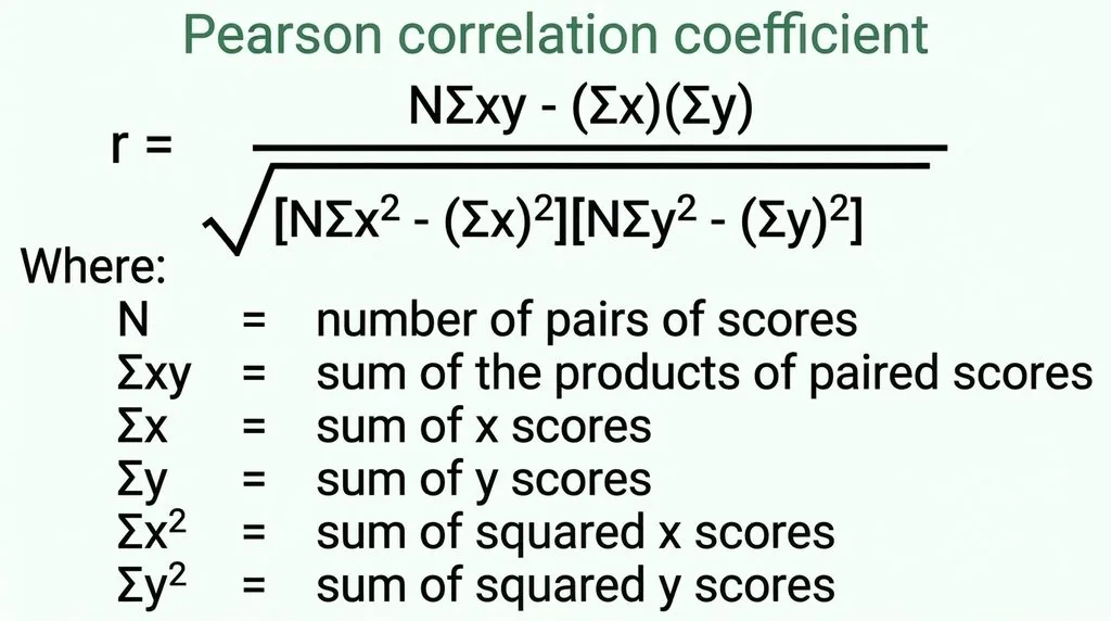

Pearson’s correlation coefficient (r) measures the strength and direction of the linear relationship between two continuous variables, on a scale from −1 to +1. +1 means a perfect positive straight-line relationship, −1 means a perfect negative one, and 0 means no linear relationship at all. You calculate it by dividing the covariation of the two variables (how they move together around their means) by the product of their standard deviations — which is why the result is unitless. The most common hand-calculation formula is the raw-score version:
r = [nΣXY − (ΣX)(ΣY)] / √{[nΣX² − (ΣX)²][nΣY² − (ΣY)²]}
A full worked example, interpretation benchmarks, assumptions, significance testing, and a Pearson-vs-Spearman decision guide follow below. If you just need the number fast, a correlation calculator does it instantly — but if you want to actually understand it (or pass a stats exam), keep reading.
What Is Pearson’s Correlation Coefficient, Exactly?
Let’s start with the story, because it makes the math easier. In the 1880s, Francis Galton was studying how traits pass from parents to children — he noticed that tall parents tend to have tall children, but not as tall (a pattern he called “regression to the mean”). Around 1895, Karl Pearson, Galton’s protégé, turned that observation into a single number that could quantify how strongly two variables move together. That number is the Pearson product-moment correlation coefficient, usually just called Pearson’s r.
Here’s what it does and doesn’t tell you:
- It measures linear relationships only. If your data form a curve, r can be near zero even when a strong relationship exists.
- It ranges from −1 to +1. The sign tells you direction; the absolute value tells you strength.
- It is unitless. Correlate height in inches with weight in pounds, or height in centimeters with weight in kilograms — you get the same r.
- It is symmetric. Correlating X with Y gives the same answer as Y with X.
- It does not establish causation. A strong r means two variables move together; it says nothing about whether one causes the other.
The symbol for the population correlation is ρ (rho); the sample statistic you actually calculate from data is r. In everyday use, people call both “the correlation coefficient.”
The Two Formulas You’ll Actually Use
You’ll see Pearson’s r written in two common forms. They give the same answer — they just organize the arithmetic differently.
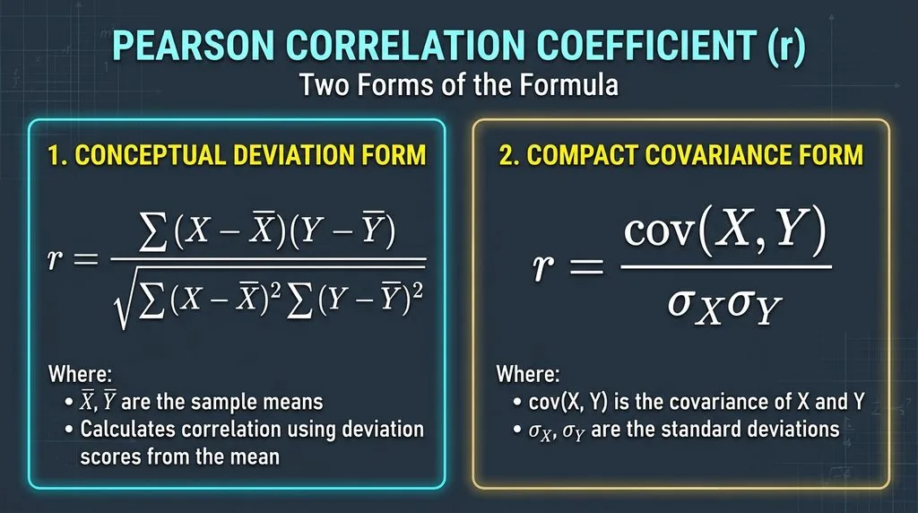
Form 1: The Deviation (Covariance) Formula
r = Σ(Xᵢ − X̄)(Yᵢ − Ȳ) / √[Σ(Xᵢ − X̄)² · Σ(Yᵢ − Ȳ)²]
This is the conceptually clean version. The numerator is the sum of cross-products of deviations: when above-average X pairs with above-average Y (and below-average with below-average), the products are positive and the sum grows — that’s a positive correlation. When one is above average and the other below, the products are negative. The denominator normalizes that sum by the spread of both variables, which squeezes the result into the −1 to +1 range and strips out the units. If you need to compute those spread terms, a standard deviation calculator handles the denominator’s building blocks.
Form 2: The Raw-Score (Computational) Formula
r = [nΣXY − (ΣX)(ΣY)] / √{[nΣX² − (ΣX)²][nΣY² − (ΣY)²]}
This is the one you use when calculating by hand, because it avoids working with decimals from the means. You only need five sums: n, ΣX, ΣY, ΣX², ΣY², and ΣXY. It’s algebraically identical to Form 1 — just rearranged.
How to Calculate the Correlation Coefficient by Hand (Full Worked Example)
Let’s say you want to know if hours of study predict exam scores. You collect data from five students:
| Student | Hours studied (X) | Exam score (Y) |
|---|---|---|
| A | 1 | 2 |
| B | 2 | 4 |
| C | 3 | 5 |
| D | 4 | 4 |
| E | 5 | 5 |
(Scaled scores for simplicity; the arithmetic works identically with real numbers.)
Step 1: Compute the five sums.
First, add three columns to your table — XY, X², Y² — and fill them in:
| Student | X | Y | XY | X² | Y² |
|---|---|---|---|---|---|
| A | 1 | 2 | 2 | 1 | 4 |
| B | 2 | 4 | 8 | 4 | 16 |
| C | 3 | 5 | 15 | 9 | 25 |
| D | 4 | 4 | 16 | 16 | 16 |
| E | 5 | 5 | 25 | 25 | 25 |
| Sum | ΣX = 15 | ΣY = 20 | ΣXY = 66 | ΣX² = 55 | ΣY² = 86 |
n = 5. If you want to double-check the averages first, a mean calculator gives X̄ = 3 and Ȳ = 4.
Step 2: Plug into the numerator.
Numerator = nΣXY − (ΣX)(ΣY) = 5(66) − (15)(20) = 330 − 300 = 30
Step 3: Plug into the denominator.
First bracket: nΣX² − (ΣX)² = 5(55) − (15)² = 275 − 225 = 50
Second bracket: nΣY² − (ΣY)² = 5(86) − (20)² = 430 − 400 = 30
Denominator = √(50 × 30) = √1500 ≈ 38.73
Step 4: Divide.
r = 30 / 38.73 = 0.775
So the correlation between study hours and exam scores in this sample is r = 0.775 — a strong positive linear relationship. Squaring it gives r² = 0.60, meaning about 60% of the variation in exam scores is explained by variation in study hours (we’ll come back to r²).
Common arithmetic pitfalls when calculating by hand:
- Forgetting to square the sum (ΣX)² — that’s different from the sum of squares ΣX². Mixing them up is the #1 hand-calculation error.
- Using n instead of n−1 in the deviation formula. (The raw-score formula above uses n directly; the (n−1) terms cancel out, which is why it’s simpler.)
- Rounding intermediate values too early. Keep 3–4 decimals until the final step.
Interpreting r: Direction, Strength, and r²
A single r value carries two pieces of information, and you need both.
Direction (the sign)
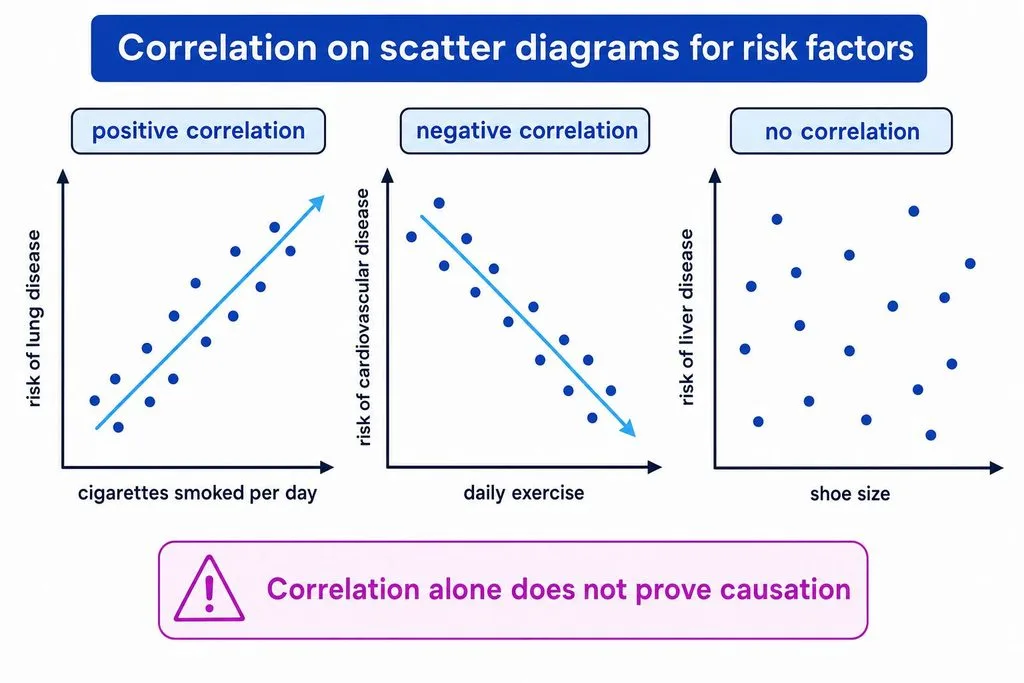
- Positive r (+): As X goes up, Y tends to go up. Example: hours studied and exam score.
- Negative r (−): As X goes up, Y tends to go down. Example: outdoor temperature and heating bill.
- r = 0: No straight-line relationship. Example: shoe size and IQ in the general population.
Strength (the absolute value)
These are conventional benchmarks, not universal laws — what counts as “strong” depends on your field. In particle physics, r = 0.3 can be remarkable; in psychology, r = 0.7 might be routine.
| |r| | Strength label |
|---|---|
| 0.00 | No linear relationship |
| 0.01 – 0.29 | Weak |
| 0.30 – 0.49 | Moderate |
| 0.50 – 0.74 | Strong |
| 0.75 – 0.99 | Very strong |
| 1.00 | Perfect |
r²: The Coefficient of Determination
Squaring r gives you you the coefficient of determination, which is far more interpretable than r itself. It tells you the proportion of variance in one variable that is “explained by” (statistically shared with) the other.
| r | r² | Variance shared |
|---|---|---|
| 0.30 | 0.09 | 9% |
| 0.50 | 0.25 | 25% |
| 0.70 | 0.49 | 49% |
| 0.775 | 0.60 | 60% |
| 0.90 | 0.81 | 81% |
This is why “r = 0.8 is twice as strong as r = 0.4” is wrong — the relationship is quadratic, not linear. Always report r² alongside r. If you want to go one step further and actually predict Y from X, that’s simple linear regression, and a regression calculator gives you the slope and intercept directly.
The 5 Assumptions of Pearson’s r (Check Before You Trust It)
Pearson’s r will calculate on almost any two columns of numbers. That doesn’t mean the result means anything. Before you interpret r, verify all five:
| # | Assumption | What it requires | How to check | If violated |
|---|---|---|---|---|
| 1 | Continuous data | Both variables interval or ratio scale (e.g., height, income, test score) | Check measurement scale | Use Spearman for ordinal |
| 2 | Linear relationship | The scatterplot forms a straight-line cloud, not a curve | Plot the data | Transform data or use Spearman |
| 3 | Approximate normality | Both variables roughly normal (matters for p-values) | Histogram, Q-Q plot | Use Spearman or bootstrap |
| 4 | Homoscedasticity | Spread of Y is constant across X (no funnel shape) | Scatterplot inspection | Transform or use robust methods |
| 5 | Independent observations | Each data pair independent of the others | Study design | Use mixed/paired models |
Plus one non-negotiable: no influential outliers. A single extreme point can swing r dramatically. Always identify outliers before computing. If you spot one, run r with and without it — if the conclusion changes, report both.
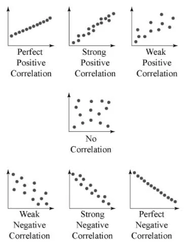
The single best way to check assumptions 2, 4, and the outlier condition at once is to look at a scatterplot before you calculate anything. A scatter plot maker lets you visualize your pairs in seconds. r is a summary of a picture — if the picture is curved or funnel-shaped or has a rogue point, the summary lies.
Pearson vs Spearman vs Kendall: Which One Should You Use?
This is the decision that trips up most students and even some researchers. Here’s the plain-English guide.
| Pearson’s r | Spearman’s ρ (rho) | Kendall’s τ (tau) | |
|---|---|---|---|
| Measures | Linear relationship | Monotonic relationship (consistent direction, any shape) | Monotonic concordance (pairwise) |
| Data type | Continuous (interval/ratio) | Ordinal or continuous | Ordinal or continuous |
| Robust to outliers? | No — very sensitive | Yes | Yes |
| Requires normality? | For p-values | No | No |
| Best for | Straight-line relationships, regression context | Curved-but-consistent trends, ranked data, outliers | Small samples, many tied ranks |
| How it computes | Raw values | Ranks of values | Pairwise concordant/discordant counts |
The decision rule in one sentence: If your scatterplot shows a straight-line cloud and your data are continuous with no wild outliers, use Pearson. If the trend is consistently upward or downward but curved, or you have outliers or ordinal/ranked data, use Spearman. If you have a small sample with lots of tied ranks, use Kendall’s tau. A solid Pearson Spearman Kendall comparison walks through the math if you want the details.
Important: “monotonic” doesn’t mean “linear.” A relationship where Y always increases as X increases — but faster at first, then slower — is monotonic but not linear. Pearson will underestimate it; Spearman will capture it.
Statistical Significance: Is Your r “Real” or Just Luck?
An r of 0.50 from n = 5 could easily be noise. The same r from n = 50 is almost certainly real. That’s why you test significance.
The t-test for correlation:
t = r × √[(n − 2) / (1 − r²)], with df = n − 2
For our worked example: r = 0.775, n = 5, df = 3.
t = 0.775 × √[3 / (1 − 0.60)] = 0.775 × √(3/0.40) = 0.775 × √7.5 = 0.775 × 2.739 = 2.12
With df = 3, the critical t for α = 0.05 (two-tailed) is about 3.18 — so our r = 0.775, despite looking strong, is not statistically significant at p < 0.05 because the sample is tiny. That’s the single most important lesson: a big-looking r from a small sample proves nothing. Always report r, df (which equals n−2), and the p-value together.
Two warnings about significance:
- With very large samples (n > 1,000), even r = 0.05 becomes “statistically significant.” That doesn’t make it meaningful — check r² and the real-world size of the effect.
- Significance ≠ strength. A result can be highly significant (tiny p-value) but weak (small r), especially with big data.
The Six Classic Mistakes People Make with Correlation
These are the errors that show up in homework, in published papers, and in viral news stories. Learn them once.
- Correlation ≠ causation. Ice cream sales and drowning deaths both rise in summer — but neither causes the other; temperature causes both. A strong r never, by itself, proves cause and effect.
- Ignoring nonlinearity. Pearson’s r measures straight-line relationships only. A perfect U-shape (like anxiety vs performance — too little or too much anxiety both hurt) can give r ≈ 0 even though a strong relationship exists. Always plot first.
- Outlier distortion. One extreme point can flip r from +0.2 to +0.8. Check for them and report sensitivity.
- Restricted range. If you correlate SAT score with college GPA but only look at students at an elite university (narrow SAT range), you’ll underestimate the true correlation. Range restriction shrinks r toward zero.
- Confusing significance with strength. “p < 0.001” means the correlation is unlikely to be zero — it says nothing about how big it is. With n = 10,000, r = 0.03 is “highly significant” but practically meaningless.
- Using Pearson on the wrong data. Ordinal data (Likert scales, ranks), categorical data, or heavily skewed variables violate the assumptions. Use Spearman or Kendall instead.
How to Report Pearson’s r (APA Style)
Journal reviewers and thesis committees expect a specific format. A complete report looks like this:
“Hours studied and exam score showed a strong positive correlation that was not statistically significant, r(3) = 0.78, p = 0.12, r² = 0.60.”
The number in parentheses after r is the degrees of freedom (n − 2). Round r to two decimal places. Report the exact p-value when you can (p = 0.12), not just “p > 0.05.” And always include r² so readers can judge the practical size, not just the statistical significance.
Quick Reference Cheat Sheet (Bookmark This)
| Item | Value / Formula |
|---|---|
| Range of r | −1 to +1 |
| Raw-score formula | r = [nΣXY − (ΣX)(ΣY)] / √{[nΣX² − (ΣX)²][nΣY² − (ΣY)²]} |
| Sums needed | n, ΣX, ΣY, ΣXY, ΣX², ΣY² |
| Degrees of freedom | df = n − 2 |
| Significance test | t = r√[(n−2)/(1−r²)], df = n−2 |
| Coefficient of determination | r² = r × r |
| Strong correlation convention | |r| ≥ 0.50 |
| Use Pearson when | Continuous, linear, no outliers, roughly normal |
| Use Spearman when | Ordinal, monotonic, outliers, curved |
| Use Kendall when | Small sample, many tied ranks |
| #1 mistake | Assuming correlation = causation |
Frequently Asked Questions
1. What is the formula for Pearson’s correlation coefficient?
The most common hand-calculation (raw-score) formula is r = [nΣXY − (ΣX)(ΣY)] / √{[nΣX² − (ΣX)²][nΣY² − (ΣY)²]}. The conceptual deviation form is r = Σ(X−X̄)(Y−Ȳ) / √[Σ(X−X̄)²·Σ(Y−Ȳ)²]. Both give the same result.
2. How do I calculate the correlation coefficient by hand?
Build a table with columns for X, Y, XY, X², and Y². Sum each column to get n, ΣX, ΣY, ΣXY, ΣX², and ΣY². Plug those six numbers into the raw-score formula and divide. A full worked example with verified arithmetic appears above.
3. What does an r value of 0.5 mean?
r = 0.5 is a moderate-to-strong positive correlation. Squared, r² = 0.25, meaning 25% of the variance in one variable is statistically shared with the other. The sign (+) means both variables tend to move in the same direction.
4. What is the difference between Pearson and Spearman correlation?
Pearson’s r measures linear relationships between continuous variables and is sensitive to outliers. Spearman’s rho measures monotonic relationships (consistent direction, any shape) using ranks, works with ordinal data, and is robust to outliers. Use Pearson for straight-line clouds; use Spearman for curved trends, ranked data, or outliers.
5. Can correlation be greater than 1 or less than −1?
No. Pearson’s r is mathematically bounded between −1 and +1. If your calculation gives a value outside that range, you made an arithmetic error — almost always mixing up (ΣX)² with ΣX².
6. Does a significant p-value mean the correlation is strong?
No. Statistical significance (small p-value) means the correlation is unlikely to be zero in the population. With very large samples, even r = 0.03 can be highly significant. Always check the magnitude of r and r² alongside the p-value.
7. What assumptions does Pearson’s correlation require?
Five: (1) both variables continuous (interval/ratio), (2) linear relationship, (3) approximate normality (for p-values), (4) homoscedasticity (constant variance), and (5) independent observations. Plus: no influential outliers. Check all of them with a scatterplot before interpreting r.
8. What is r squared and why does it matter?
r² (the coefficient of determination) is the square of r and tells you the proportion of variance in one variable explained by the other. r = 0.7 gives r² = 0.49 (49% explained). It’s the more interpretable measure of effect size — always report it with r.
Final Thought
Pearson’s r is one of the most used — and most misused — numbers in statistics. It’s elegant: six sums, one division, and you get a single digit between −1 and +1 that summarizes an entire cloud of points. But that elegance is also the danger: one number can’t tell you about curves, outliers, restricted ranges, or causation. Calculate it correctly (use the worked example above to check your arithmetic), verify the assumptions, report r, df, p, and r² together — and always, always look at the scatterplot first. Do that, and you’ll be ahead of most people who ever quote a correlation.